Walkthrough

Learning Objectives

At the end of this learning activity you will be able to:

• Relate the null-hypotheses of chi2 tests, t-tests, ANOVAs, and Krustal-Wallace H-tests.

• Calculate cross-tabulations of two categorical variables using pd.crosstab.

• Employ pg.chi2_independence to estimate the correlation between two categorical variables.

• Describe how to test if a distribution is normally distributed using multiple methods.

• Employ pg.ttest, pg.anova, and pg.kruskal to look for differences in a dependent variable between different categorical variables.

• Utilize post-hoc tests to refine the answer of an ANOVA.

Introduction

As we discussed with Dr. Devlin in the introduction video, this week and next we are going to look at HIV neurocognitive impairment data from a cohort here at Drexel. Each patient was given a full-scale neuropsychological exam and the resulting values were aggregated and normalized into Z-scores based on demographically matched healthy individuals.

In this walkthrough we will explore the demographic variables within this dataset to practice different types of hypothesis testing. In the lab you will dive deeper and explore the effects of antiretroviral medications on neurological impairment. In this cohort, we have two major drug regimens, d4T (Stavudine) and the newer Emtricitabine/tenofovir (Truvada). The older Stavudine is suspected to have neurotoxic effects that are not found in the newer Truvada. We will use inferential statistics to understand this effect.

Hypothesis Testing

Hypothesis testing is a type of inferential statistics in which one compares a distribution to a previously assumed null model that represents the simplest explanation of the world. The process of the test then involves rigorously evaluating the likelihood of observing this dataset under that null assumption. If, after rigorous evaluation, we find that the likelihood of generating this dataset under null model is below some threshold (ie p<0.05) we reject the null hypothesis and accept the alternative.

While one can test arbitrarily complicated hypotheses, in biology we tend to fall back on a few go-to tests:

• 2-factor tests (chi2-tests)

• Tests of means (t-tests, ANOVAs, etc.)

• Correlations (linear regression)

We’ll cover the first two this week, and the last next week.

When boiled down, all of these tests rigorously balance four things:

• Effect size : How large is difference observed divided by the spread of the observations.

• Type 1 Error (false-positives, p-value) : The likelihood of incorrectly rejecting the null hypothesis.

• Type 2 Error (false-negatives, power) : The likelihood of incorrectly accepting the null hypothesis.

• Number of observations.

Pingouin

The pingouin Python package is a statistical tool designed to bridge the gap between the data manipulation capabilities of pandas and the visualization strengths of seaborn, with a specific focus on ease of use and accessibility. It is particularly tailored towards researchers who are embarking on their journey into data exploration and biostatistics, leveraging their familiarity with pandas for data manipulation and seaborn for data visualization.

pingouin is built on top of pandas DataFrame objects, which means that it integrates seamlessly with the pandas ecosystem. This allows users to effortlessly prepare their data using pandas and then apply statistical tests and models using pingouin. The package offers a wide range of statistical functions, including t-tests, ANOVAs, correlation tests, and regression analyses, with a syntax that is more intuitive and less verbose than some of its counterparts. This makes pingouin an attractive option for biologists who may not have a deep background in statistics but need to conduct sophisticated statistical analyses as part of their research.

Two other popular packages for statistical analysis in python are scipy.stats and statsmodels. Scipy offers many low-level functions for calculating basic statistical tests like t-tests, ANOVAs, Mann-Whitney, etc. However, these low level functions require extensive programming knowledge to leverage properly.

Statsmodels offers a wealth of complex statistical modeling, p-value correction tools, and allows arbitrarily complicated regression analysis. However, due to its complexity, it is not approachable for beginners.

Under the hood, Pingouin employs scipy.stats, statsmodels, and a number of other tools into a simple and intuitive API designed to be user-friendly and accessible. The outputs it creates are interpretable at a glance and contain outputs from a number of lower-level tools. This is intended to make it easier to apply statistical tests and interpret their results without getting bogged down in the complexities of statistical theory. Additionally, pingouin is designed to work well with Pandas and the Jupyter Notebook environment, which is popular among scientists for interactive data analysis.

Check out the documentation for Pingouin.

• Quick Start Examples

• Available tests

• Which test to pick

import numpy as np
import seaborn as sns
import pandas as pd
import matplotlib.pyplot as plt

import pingouin as pg

%matplotlib inline

data = pd.read_csv('hiv_neuro_data.csv')
data['education'] = data['education'].astype(float)
data.head()

	sex	age	education	race	processing_domain_z	exec_domain_z	language_domain_z	visuospatial_domain_z	learningmemory_domain_z	motor_domain_z	ART	YearsSeropositive
0	male	62	10.0	AA	0.5	0.6	0.151646	-1.0	-1.152131	-1.364306	Stavudine	13
1	male	56	10.0	AA	-0.5	1.2	-0.255505	-2.0	-0.086376	-0.348600	Truvada	19
2	female	51	10.0	AA	0.5	0.1	0.902004	-0.4	-1.139892	0.112215	Stavudine	9
3	female	47	12.0	AA	-0.6	-1.2	-0.119866	-2.1	0.803619	-2.276768	Truvada	24
4	male	46	13.0	AA	-0.4	1.3	0.079129	-1.3	-0.533607	-0.330541	Truvada	14

When studying HIV Associated Neurocognitive Disorder (HAND) we measure a number of cognitive domains through a ~90 min test battery. The results of these tests are then aggregated into 6 cognitive domains.

• Speed of Information Processing : processing_domain_z : How quickly an individual can understand and react to the information being presented. This domain evaluates the speed at which cognitive tasks can be performed, often under time constraints.

• Learning and Memory : learningmemory_domain_z : This involves both the acquisition of new information (learning) and the ability to retrieve this information over time (memory). It includes both verbal learning and memory (e.g., remembering words or stories) and visual learning and memory (e.g., remembering shapes or patterns).

• Executive Function : exec_domain_z : The complex cognitive processes required for planning, organizing, problem-solving, abstract thinking, and executing strategies. This domain also encompasses decision-making and cognitive flexibility, which is the ability to switch between thinking about two different concepts or to think about multiple concepts simultaneously.

• Motor Skills : motor_domain_z : This domain assesses the coordination, speed, and dexterity of motor movements, including both fine motor skills (e.g., hand movements, writing) and gross motor skills (e.g., walking, coordination).

• Language Skills : language_domain_z : The ability to understand and produce language. While not always as prominently affected in HAND as other cognitive domains, assessments might include naming, fluency, and comprehension tasks.

• Sensory-Perceptual Skills : visuospatial_domain_z : Although less commonly assessed in HAND research, this domain involves the ability to interpret sensory information, including visual and auditory processing.

The outcomes of these test are highly correlated with age, sex, race, and education. This makes it difficult to compare the raw results of a test between individuals across these covariates; ie. is this 65 year old performing worse on a memory task relative to a 25 year old because of their age or because of some type of impairement? With the raw scores alone, this is impossible.

However, if we collect data from a large number of presumably healthy individuals we can create a normalization scale. These are normalized to a Z-scale. In a z-scaled value, z = 0 is the mean; all individuals performing at the average of covariate matched controls will have a score of 0. Each unit of a z-scale is 1-standard-deviation. An individual with a z = 1 is performing 1 standard-deviation above thier peers while a z = -1.5 implies that they are performing 1.5 stds below their matched peers.

You’ve probably heard of this before: an IQ score works in a similar way. It uses a standard scale. This has a mean of 100 and a standard deviation of 10. An average IQ is 100 (by definition). An IQ of 210 (Marylin vos Savant) is 11 standard-deviations above an average individual.

Categorical comparisons

Q1: Count the number of participants of each sex and race.

q1_race_counts = data['race'].value_counts() # SOLUTION
q1_sex_counts = data['sex'].value_counts() # SOLUTION

grader.check("q1_demographic_breakdown")

Once we have the counts, we can change each into a probability. This represents the likelihood of observing any given instance of the categorical variable. We can think of this like an unfiar set of dice.

q1_race_counts/q1_race_counts.sum()

race
AA    0.676923
C     0.227692
H     0.095385
Name: count, dtype: float64

q1_sex_counts/q1_sex_counts.sum()

sex
male      0.692308
female    0.307692
Name: count, dtype: float64

Let’s do the same thing for the ART column.

art_counts = data['ART'].value_counts()
art_counts/art_counts.sum()

ART
Stavudine    0.52
Truvada      0.48
Name: count, dtype: float64

I wonder if there is a relationship between demographic variables and ART therapy?

That was looking at each measurement individually, if we want to know whether they are correlated, we need a different type of table. We need a table that measures the number of occurances of male & Stavudine, female & Stavudine, male & Truvada, female & Truvada, etc. This is often called a cross tabulation. Traditionally one would use a set of for-loops to count this data, but Pandas has a tool for exactly this purpose.

pd.crosstab(data['sex'], data['ART'], margins=True)

ART	Stavudine	Truvada	All
sex
female	53	47	100
male	116	109	225
All	169	156	325

It can also give us frequencies.

pd.crosstab(data['race'], data['ART'], margins=True, normalize='all')

ART	Stavudine	Truvada	All
race
AA	0.313846	0.363077	0.676923
C	0.153846	0.073846	0.227692
H	0.052308	0.043077	0.095385
All	0.520000	0.480000	1.000000

Hypothesis Testing

When testing the correlation between two categorical variables we want to use a chi2 test. It has the null hypothesis that the two categorical distributions are uncorrelated. Rejection of that hypothesis (ie p<0.05) indicates there is some linkage between the two distributions.

Notes:

In your cross tabulation table you need at least 5 observations in each cell. Fewer than that can lead to significant losses in statistical power.

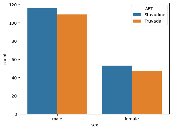
When we want to visualize a categorical comparison, it is best to use a countplot that uses both x and hue to show the two factors. If there is a difference, we will see that the bars have inconsistent relative heights when compared to each other.

sns.countplot(data = data,
              x = 'sex',
              hue = 'ART')

<Axes: xlabel='sex', ylabel='count'>

Pingouin has a function for performing a chi2 test from a pd.Dataframe directly: pg.chi2_independence. It will return three things:

# Pingouin does the crosstab internally, it just wants the df and columns

expected, obs_cor, stats = pg.chi2_independence(data, 'sex', 'ART')

If these two variables were randomly associated, what would I have gotten?

expected

ART	Stavudine	Truvada
sex
female	52.0	48.0
male	117.0	108.0

What did I actually observe after correction?

obs_cor

ART	Stavudine	Truvada
sex
female	52.5	47.5
male	116.5	108.5

What is the likelihood that obs_cor is different from expected?

stats

	test	lambda	chi2	dof	pval	cramer	power
0	pearson	1.000000	0.014468	1.0	0.904260	0.006672	0.051659
1	cressie-read	0.666667	0.014468	1.0	0.904258	0.006672	0.051659
2	log-likelihood	0.000000	0.014470	1.0	0.904253	0.006673	0.051659
3	freeman-tukey	-0.500000	0.014471	1.0	0.904249	0.006673	0.051659
4	mod-log-likelihood	-1.000000	0.014472	1.0	0.904244	0.006673	0.051659
5	neyman	-2.000000	0.014475	1.0	0.904235	0.006674	0.051660

p ~= 0.9, therefore we cannot reject the hypothesis that ART therapy is unrelated to sex.

Q2: Is race and education correlated in this dataset?

# Bin education into three bins:
#  * Up to HS education (0, 12]
#  * HS-4yr College (12, 16]
#  * >4yr College (16, np.inf]
# pandas has a function pd.cut that that accomplish this.

# Add this column back into the dataframe as a new column called `education_binned`
data['education_binned'] = pd.cut(data['education'], [0, 12, 16, np.inf])

# Calculate the chi2 test between race and education_binned
q2_expected, q2_obs_cor, q2_stats = pg.chi2_independence(data, 'race', 'education_binned') # SOLUTION NO PROMPT

# Is race and education correlated? (yes or no)
q2_pval_ans = 'yes' # SOLUTION

# Are there "more" or "less" H's with 12-16 years of education than we'd expect by chance
q2_inter_ans = 'less' # SOLUTION

grader.check("q2_demographic_education")

So, we found that there is a link between race and education, with AA and H individuals have less people in the higher education brackets and more in the lower education brackets.

In this instance we used stratification to split education into categorical variables representing meaningful cutoffs. We can also keep the education value as a continious measurement and compare across categories.

Continious comparisons

In order to choose the right test we need to walk down a set of decision trees to find the appropriate answer. There are a number of places you can find these decision trees (or you can make your own), we’ll use the one from the pingouin tool.

https://pingouin-stats.org/build/html/guidelines.html

The first thing to test: normality.

If the variable is normally distributed (or can be approximated as normal) we can use more powerful parametric tests. If it is not normal, we need to use non-parametric tests.

A qqplot is a common way to visualize the fit between an observed distribution and a theoretical one. It plots the observed data against a desired distribution (usaually the normal distribution). If there is strong agreement, it likely means the data fits the distribution. It is the best place to start when starting considering normality.

pg.qqplot(data['education'], dist='norm')

<Axes: xlabel='Theoretical quantiles', ylabel='Ordered quantiles'>

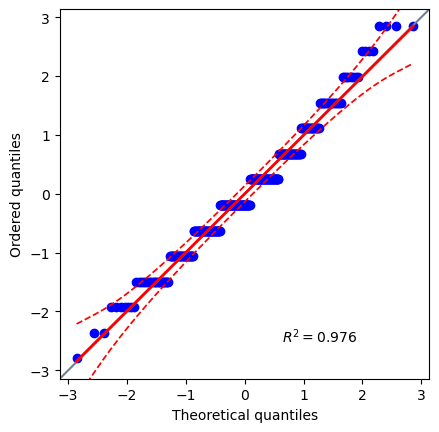
Extremely high agreement. I would expect this to be normally distributed. Let’s use Pingouin to test it.

# Tests the null-hypothesis: is this derived from a normal distribution
# with the default parameters

pg.normality(data['education'])

	W	pval	normal
education	0.975734	0.000027	False

Interesting, it rejected the hypothesis that this data is normally distributed. This is why you NEED to have documentation open when utilizing these tools.

https://pingouin-stats.org/build/html/generated/pingouin.normality.html

method: str Normality test.

• ‘shapiro’ (default) performs the Shapiro-Wilk test using scipy.stats.shapiro(),

• ‘normaltest’ performs the omnibus test of normality using scipy.stats.normaltest(),

• ‘jarque_bera’ performs the Jarque-Bera test using scipy.stats.jarque_bera().

The Omnibus and Jarque-Bera tests are more suitable than the Shapiro test for large samples.

pg.normality(data['education'], method='normaltest')

	W	pval	normal
education	5.843312	0.053844	True

pg.normality(data['education'], method='jarque_bera')

	W	pval	normal
education	5.585359	0.061257	True

Now we see that both of these methods, and the qq-plot agree that this data is normally disitributed.

Two group measurement

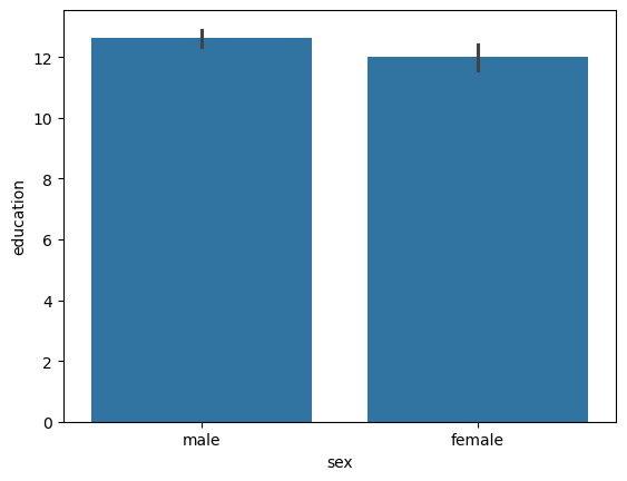
sns.barplot(data = data,
            x = 'sex',
            y = 'education')

<Axes: xlabel='sex', ylabel='education'>

Handy-dandy t-test. Measures the null-hypothesis:

• One-sample: Does this sample have a mean of mu?

• Two-sample (independent): Do these two distribution have the mean value?

• Two-sample (paired): Do these pre/post measurements of the same sample have the same mean value?

male_edu = data.query('sex == "male"')['education']
female_edu = data.query('sex == "female"')['education']
pg.ttest(male_edu, female_edu)

	T	dof	alternative	p-val	CI95%	cohen-d	BF10	power
T-test	2.245961	202.108089	two-sided	0.025789	[0.07, 1.13]	0.263056	1.438	0.587972

Breaking this down:

• T = 2.245961 : Called the T-statistic : (mean_M-mean_F)/std_P*sqrt(1/N_m+1/N_f)

• dof = 202.1 : The number of samples after dropping missing and applying corrections.

• alternative = two-sided : The mean of females can be larger or smaller than males.

• p-val = 0.025 : The likelihood of seeing this difference by chance.

• CI95% = [0.07, 1.13] : The difference in means between males and females is between 0.7 and 1.13 years.

• cohen-d = 0.26 : The effect size : (mean_M-mean_F)/std_P

• BF10 = 1.43 : Bayes Factor : P(D|H1)/P(D|H0) : The likelihood of the data given the alternative hypothesis divided by the likelihood of the data under the null hypothesis.

• power = 0.587 : The likelihood of see an effect if there truly was one given cohen-D and dof.

Multi-group measurement

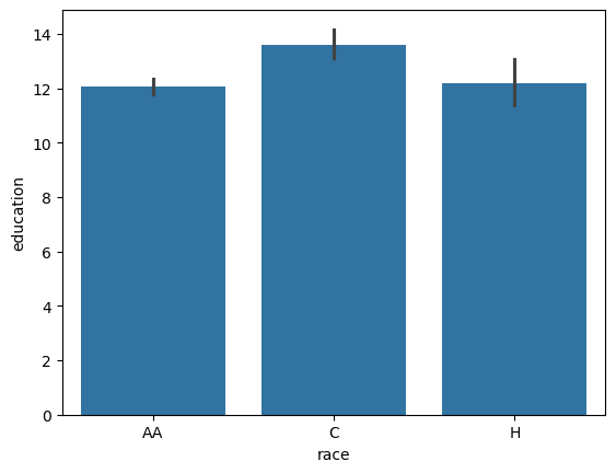
sns.barplot(data = data,
            x = 'race',
            y = 'education')

<Axes: xlabel='race', ylabel='education'>

Handy-dandy One-way ANOVA with post-hoc tests.

https://pingouin-stats.org/build/html/guidelines.html#anova

# First test for equal variances to pick correct ANOVA

pg.homoscedasticity(data, dv='education', group='race')

	W	pval	equal_var
levene	1.292877	0.275901	True

pg.anova(data, dv='education', between='race', detailed=True)

	Source	SS	DF	MS	F	p-unc	np2
0	race	131.796715	2	65.898357	13.37776	0.000003	0.076717
1	Within	1586.160208	322	4.925963	NaN	NaN	NaN

Here the ANOVA rejects the hypothesis that the mean is the same across races. However, it does not tell us which ones are different. That’s where post-hoc testing comes in. Since we have equal-varainces across the group, it suggets Tukey’s post hoc test.

pg.pairwise_tukey(data=data, dv='education', between='race')

	A	B	mean(A)	mean(B)	diff	se	T	p-tukey	hedges
0	AA	C	12.077273	13.608108	-1.530835	0.298258	-5.132588	0.000001	-0.697499
1	AA	H	12.077273	12.193548	-0.116276	0.425785	-0.273085	0.959729	-0.054118
2	C	H	13.608108	12.193548	1.414560	0.474836	2.979050	0.008714	0.567577

This provided a table with a row for each comparison. p-tukey indicates the rows with significant differences.

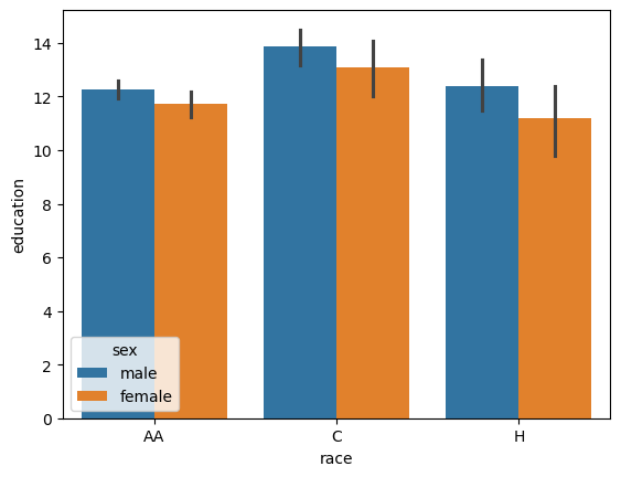
We can also do Multi-way ANOVAs; this is where you have more than one independent variable splitting your data. Here, we can look at how both race and gender impact educational attainment.

sns.barplot(data = data,
            x = 'race',
            hue = 'sex',
            y = 'education')

<Axes: xlabel='race', ylabel='education'>

pg.anova(data, dv='education', between=['race', 'sex'], detailed=True)

	Source	SS	DF	MS	F	p-unc	np2
0	race	133.744087	2.0	66.872043	13.700951	0.000002	0.079104
1	sex	27.055406	1.0	27.055406	5.543195	0.019158	0.017080
2	race * sex	2.119345	2.0	1.059672	0.217109	0.804961	0.001359
3	Residual	1556.985457	319.0	4.880832	NaN	NaN	NaN

This tells us that there is likely a difference between race, between sex, but there likely isn’t an interactive term. We can also do the post-hoc tests across all comparisons.

results = pg.pairwise_tests(data=data, dv='education', between=['race', 'sex'])
results

	Contrast	race	A	B	Paired	Parametric	T	dof	alternative	p-unc	BF10	hedges
0	race	-	AA	C	False	True	-4.794172	110.376193	two-sided	0.000005	5562.177	-0.697499
1	race	-	AA	H	False	True	-0.247486	36.168163	two-sided	0.805932	0.209	-0.054118
2	race	-	C	H	False	True	2.658937	55.713740	two-sided	0.010214	4.718	0.567577
3	sex	-	female	male	False	True	-2.245961	202.108089	two-sided	0.025789	1.438	-0.262445
4	race * sex	AA	female	male	False	True	-1.826097	149.778935	two-sided	0.069827	0.739	-0.254068
5	race * sex	C	female	male	False	True	-1.230186	41.659681	two-sided	0.225529	0.481	-0.313088
6	race * sex	H	female	male	False	True	-1.322973	8.498605	two-sided	0.220332	0.753	-0.461862

results.loc[results['p-unc'] < 0.05]

	Contrast	race	A	B	Paired	Parametric	T	dof	alternative	p-unc	BF10	hedges
0	race	-	AA	C	False	True	-4.794172	110.376193	two-sided	0.000005	5562.177	-0.697499
2	race	-	C	H	False	True	2.658937	55.713740	two-sided	0.010214	4.718	0.567577
3	sex	-	female	male	False	True	-2.245961	202.108089	two-sided	0.025789	1.438	-0.262445

If we had repeated measures for individuals (ie biological replicates) we can also add , within = 'sample'. This would help correct for within sample variability.

Non-parametric comparisons

Q3: Use the appropriate non-parametric method.

Let’s pretend that we believed the first Shapiro-Wilk normality test and instead used non-parametric methods. Use the flowchart below to test the whether there is a difference in education level across race.

https://pingouin-stats.org/build/html/guidelines.html#non-parametric

Points	5
Public Checks	4

Points: 5

# Use the appropriate test from the Guidelines
q3_stats = pg.kruskal(data, dv='education', between='race') # SOLUTION
q3_stats

	Source	ddof1	H	p-unc
Kruskal	race	2	22.498491	0.000013

# Use the appropriate post-hoc test from the Guidelines
q3_post_hoc = pg.pairwise_tests(data, dv='education', between='race', parametric=False) # SOLUTION
q3_post_hoc

	Contrast	A	B	Paired	Parametric	U-val	alternative	p-unc	hedges
0	race	AA	C	False	False	5199.0	two-sided	0.000003	-0.697499
1	race	AA	H	False	False	3482.0	two-sided	0.848419	-0.054118
2	race	C	H	False	False	1540.5	two-sided	0.005371	0.567577

Compare this answer to the parametric method.

# Are they the 'same' or 'different'

q3_comparison = 'same' # SOLUTION

grader.check("q3_nonparametric")

We should see that we’ll get the same answer between parametric and non-parametric methods.

We’ve now seen a handful of methods for testing the difference between populations. In the lab, you will use these skills to test the effects of different ART drugs on neurocognitive impairment.

---

grader.check_all()